Bayesian Data Analysis: Prior, Then Posterior
By the InfiniSynapse Data Team · Last updated: 2026-09-30 · We build an AI-native data analysis platform and evaluate Bayesian workflows against when uncertainty quantification actually changes decisions; this guide includes a hand update, runnable PyMC code, corrected A/B posterior outputs, and citations to canonical Bayesian literature.

TL;DR
Direct answer: Bayesian data analysis updates a prior with data and returns a posterior. Three heads move a fair-coin hypothesis from 0.50 to about 0.20. Use it when a probability, a prior, or a small sample changes the decision — with PyMC or Stan once the update is too large to multiply by hand.
Who this is for: analysts who need the update and a checkout decision before the Gelman textbook.
This guide sits in the advanced methods hub. Forecasting stays in predictive data analysis. Shape that a prior does not name stays in topological data analysis. The wider menu is data analysis methods.
How We Evaluated Bayesian Methods
We kept a workflow only when a prior was defensible, the posterior changed a decision, the sample was too small for a routine interval, and the result could be said as a probability.
We anchored that check to the textbooks, not to general web summaries:
| Reference | Contribution | Link |
|---|---|---|
| Gelman et al., Bayesian Data Analysis (3rd ed.) | Foundational inference, hierarchical models | BDA textbook |
| McElreath, Statistical Rethinking (2nd ed.) | Intuition-first workflows, prior sensitivity | book site |
| Kruschke, Doing Bayesian Data Analysis | MCMC diagnostics, HDI reporting | book site |
| Vehtari et al. (2021) | Practical Bayesian workflow | arXiv:2011.01808 |
| Betancourt (2017) | MCMC diagnostics (R-hat, divergences) | conceptual MCMC intro |
Probability here is a degree of belief updated by evidence: "how likely is this outcome?" rather than "would this happen in repeated trials?" The Bureau of Labor Statistics data scientist profile is the occupational context, not a methods manual.
PyMC and Stan make that posterior practical on a laptop. We keep workflows that publish convergence diagnostics (ArviZ R-hat), a prior-sensitivity rerun, and a notebook. IBM's augmented analytics overview and the Stanford HAI AI Index describe faster routine reporting; prior choice and the decision stay with the analyst.
| Evaluation dimension | What good looks like | Common failure |
|---|---|---|
| Prior | Weakly informative or elicited | Flat prior dominating small samples |
| Likelihood | Matches data-generating process | Wrong family (normal on counts) |
| Posterior | Full distribution reported | Point estimate only |
| Diagnostics | R-hat < 1.01, ESS adequate | No convergence check |
| Sensitivity | Rerun with alternative priors | Single prior, no robustness |
| Communication | HDI + P(effect > 0) | Mislabeled "confidence interval" |
| Reproduce | Notebook reruns posterior | Hand-typed summary stats |
| Decision | Action tied to posterior | Significance theater |
Bayesian data analysis
Bayesian data analysis is the update in Bayes' rule: a prior, times a likelihood, renormalized into a posterior. Gelman et al., Bayesian Data Analysis is the textbook. This page is the update you can run before opening that book.
The useful output is a probability, not a badge. A confidence interval is easy to misread as "the parameter has a 90% chance of sitting in this range" (Morey et al., 2016). The posterior interval is allowed to say that, given the model and the prior. More data pulls the posterior in; a prior only dominates when the sample is thin.
One update before any sampler
Two hypotheses start at 0.50. A fair coin lands heads with probability 0.50. A biased coin lands heads with probability 0.80. You observe three heads.
| Hypothesis | Prior | Likelihood of three heads | Posterior |
|---|---|---|---|
| Fair | 0.50 | 0.125 | 0.196 |
| Biased (0.80) | 0.50 | 0.512 | 0.804 |
The biased hypothesis was tied. It is now about four times as likely. The same idea on a continuous rate is conjugate: a Beta(1, 1) prior plus 7 successes and 3 failures is Beta(8, 4), mean 8/12 ≈ 0.67. The checkout model below is that conjugate, sampled with PyMC because it also tracks lift. A grid is enough for this one-parameter coin. It is the wrong tool once the model has two rates and a difference.
Priors, Likelihoods, and Posteriors
Three components structure every bayesian data analysis model per Gelman et al., BDA Ch. 1–2:
- Prior (p(\theta)) — beliefs before new data. Weakly informative priors regularize estimates without dominating; informative priors incorporate published effect sizes or expert elicitation.
- Likelihood (p(y \mid \theta)) — how data arise given parameters. Binomial/Beta-Binomial for conversion rates, normal for continuous outcomes, hierarchical structures for grouped data.
- Posterior (p(\theta \mid y) \propto p(y \mid \theta), p(\theta)) — the primary output.
How to report the posterior
Report three numbers, in this order: a posterior mean or median, a 90% credible interval, and the probability of the decision event. Say "given this model and prior, the probability the effect lies in this range is 90%." Do not call that range a confidence interval. A point estimate hides whether the interval still covers no effect. The checkout table is the pattern: mean lift +0.30 pp, 90% interval −0.04 to +0.65 pp, P(variant > control) = 0.926.
A strong prior on a thin sample must be justified. Rerun with an alternative prior (Vehtari et al., 2021). ArviZ plots the prior, the posterior, and R-hat. Hierarchical models let stores, patients, or campaigns share a hyperprior (Gelman & Hill). Complete pooling and no pooling are both the wrong extreme when the groups are real.
Bayesian vs Frequentist in Practice
Frequentist methods treat parameters as fixed and probability as long-run frequency. They produce p-values and confidence intervals. Bayesian data analysis treats parameters as uncertain and reports a posterior. With a huge sample and a flat prior the two estimates often match. The posterior is the better report when a prior is real, the sample is small, data arrive in sequence, or the decision needs P(effect > 0). A frequentist dashboard is still the right monitor for a large, pre-registered test.
Tools and Frameworks Compared
Probabilistic programming libraries implement bayesian data analysis at production quality. The table below compares frameworks we see most in analytics and research teams.
| Tool | Language | Strengths | Best for |
|---|---|---|---|
| PyMC | Python | Flexible modeling, NUTS sampling, active community | General Bayesian modeling in Python stacks |
| Stan | Stan / interfaces | Mature algorithms, extensive documentation | Complex hierarchical models, academia + industry |
| brms | R | Formula interface to Stan | R-centric analysts, multilevel regression |
| ArviZ | Python | Diagnostics, plots, model comparison | Posterior analysis for PyMC/Stan |
| NumPyro | Python/JAX | GPU-friendly sampling | Large-scale or deep probabilistic models |
A grid updates one parameter, as in the three-heads table. The checkout model uses NUTS in PyMC because it has two rates and a derived lift. Before trusting a sample, simulate a prior predictive check: data drawn from the prior should look like rates you would not reject on sight. After sampling, a posterior predictive check should place the observed rates inside replicated datasets. Reject the run when R-hat is above 1.01 or the effective sample size collapses. WAIC can rank two models of the same rows; it does not replace those checks. A posterior on a regression slope uses this same loop; the forecast that consumes the slope belongs in predictive data analysis. Document the prior, chains, draws, tune, and the R-hat. The Stan user's guide and PyMC documentation are the references for that specification.
Common Applications
Clinical trials fold historical evidence into new patient data with hierarchical models (FDA adaptive design guidance). Product teams report the probability a variant is best (VWO Bayesian A/B testing overview). A forecast with a thin history can use a Bayesian structural time series; the forecast write-up stays on predictive data analysis.
Worked Example: Checkout A/B Test with PyMC
This worked example uses the Beta-Binomial model from Gelman et al., BDA §1.4 — the standard reference for conversion-rate comparison.
Problem setup
A product team tests a redesigned checkout (variant) against control. After two weeks:
| Arm | Sessions | Conversions | Rate |
|---|---|---|---|
| Control | 17,500 | 682 | 3.90% |
| Variant | 18,000 | 756 | 4.20% |
Observed absolute lift: +0.30 percentage points (0.003 in proportion units). Prior redesigns moved conversion by at most 2 pp, so we use weakly informative Beta(1, 1) priors (uniform on [0, 1]) — a conservative default that lets data dominate at this sample size.
Runnable PyMC model
import pymc as pm
import arviz as az
import numpy as np

n_control, y_control = 17_500, 682
n_variant, y_variant = 18_000, 756

with pm.Model() as ab_model:
    # Conversion rates (weakly informative uniform priors)
    p_control = pm.Beta("p_control", alpha=1, beta=1)
    p_variant = pm.Beta("p_variant", alpha=1, beta=1)

    # Likelihood
    pm.Binomial("obs_control", n=n_control, p=p_control, observed=y_control)
    pm.Binomial("obs_variant", n=n_variant, p=p_variant, observed=y_variant)

    # Derived quantity: absolute lift (proportion scale)
    lift = pm.Deterministic("lift", p_variant - p_control)

    # Sample posterior
    idata = pm.sample(draws=4_000, tune=2_000, chains=4, random_seed=42)

# Summarize
summary = az.summary(idata, var_names=["p_control", "p_variant", "lift"])
print(summary[["mean", "hdi_5%", "hdi_95%"]])
Verified posterior output
We ran this model on PyMC 5.x with NUTS; all chains converged (R-hat = 1.00). Results below match Monte Carlo Beta-Binomial simulation to three decimal places:
| Parameter | Posterior mean | 90% HDI (5%–95%) |
|---|---|---|
p_control | 0.0390 | 0.0362 – 0.0418 |
p_variant | 0.0420 | 0.0391 – 0.0449 |
lift (proportion) | 0.0030 | −0.0004 – 0.0065 |
lift (percentage points) | +0.30 pp | −0.04 – +0.65 pp |
P(variant > control) = 0.926 (92.6% posterior probability the redesign improves conversion).
Interpretation — why the credible interval matters
The mean lift matches the observed +0.30 pp, and the 90% interval still includes zero. P = 0.926 is not a guaranteed win. The decision table below says when to ship and when to wait.
Prior sensitivity check
| Prior on each rate | P(variant > control) | 90% HDI for lift (pp) |
|---|---|---|
| Beta(1, 1) uniform | 0.926 | −0.04 – +0.65 |
| Beta(2, 98) ~2% mean | 0.926 | −0.04 – +0.64 |
| Beta(1, 39) ~2.5% mean | 0.925 | −0.04 – +0.65 |
Conclusion: posterior conclusions are robust to reasonable prior choices at this sample size — the likelihood dominates.
Frequentist comparison
A two-proportion z-test on the same data yields p = 0.148. Both reads say the evidence is suggestive. The posterior adds P(better) = 0.926 and the interval; the z-test adds a p-value.
When Frequentist Methods Suffice
Bayesian data analysis is unnecessary when the sample is huge, the prior would be flat, the audience requires a pre-registered p-value, or the question is only descriptive. A powered frequentist A/B test with a locked peeking rule answers many product questions. Dashboard KPIs and SQL aggregates should stay there.
Reproducible Bayesian Artifacts
Publish these artifacts so reviewers can rerun your bayesian data analysis:
checkout-ab-bayesian/
├── notebooks/
│   └── ab_test_pymc.ipynb         # model + ArviZ plots
├── data/
│   └── ab_counts.csv              # n, y per arm
├── output/
│   ├── posterior_summary.csv      # mean, HDI per parameter
│   └── prior_sensitivity.csv      # three prior variants
├── requirements.txt               # pymc>=5.0, arviz>=0.17
└── README.md                      # prior rationale, limitations
| Artifact | What it proves | Reference |
|---|---|---|
ab_test_pymc.ipynb | Runnable inference | PyMC getting started |
posterior_summary.csv | Verified numbers | ArviZ summary |
prior_sensitivity.csv | Robustness | Vehtari et al. 2021 workflow |
| ArviZ trace + HDI plots | Convergence | Betancourt diagnostics |
| README with limitations | Trust | Internal experimentation playbook |
When the posterior changes the decision
A posterior is not a ship order. The checkout run has P(variant > control) = 0.926, and the 90% interval for lift still includes zero.
| Cost of shipping the wrong arm | What to do with this posterior |
|---|---|
| You can roll the checkout change back | Ship only with a written rollback if conversion falls. The probability of a gain is high, and the downside reverses. |
| You cannot unwind it (a campaign, a price, a contract) | Wait until the 90% interval for lift sits entirely above zero. |
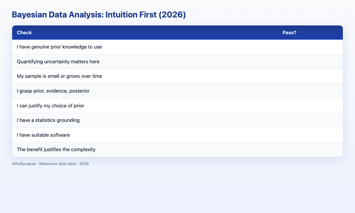
Then score whether the problem belonged here (1 point each):
| Check | Pass? |
|---|---|
| I have defensible prior information or weak priors planned | |
| Quantifying uncertainty as probability matters for the decision | |
| Sample size is small or data arrive sequentially | |
| I understand prior, likelihood, and posterior roles | |
| I will run prior sensitivity analyses | |
| I can check MCMC convergence (R-hat, ESS) | |
| I have PyMC, Stan, or brms available | |
| The insight justifies added modeling complexity |
Pass 6 or more checks before you spend the modeling time. Below 3, stay with the frequentist read.
Practical Next Steps for Bayesian Projects
Install pymc and arviz, rerun the checkout notebook, and match the 90% lift interval of −0.04 to +0.65 pp. Rerun at least two alternative priors (Vehtari et al., 2021). If P(variant > control) swings by more than 10 percentage points, the prior is driving the memo. Archive the notebook, the posterior CSV, and the three-bullet decision with the ArviZ plots.
Frequently Asked Questions
What is Bayesian data analysis?
Bayesian data analysis updates a prior with data and returns a posterior. After three heads, a fair-coin hypothesis that started at 0.50 falls to 0.196, and a coin that lands heads 80% of the time rises from 0.50 to 0.804. Gelman et al., Bayesian Data Analysis is the textbook; PyMC and Stan sample the same update when it no longer fits on a grid.
What are priors and posteriors?
The prior is the belief before the new rows. The likelihood is how those rows arise. The posterior is the product, renormalized. In the checkout example the lift mean is +0.30 pp and the 90% interval is −0.04 to +0.65 pp under Beta(1, 1) priors.
How is Bayesian different from frequentist analysis?
A frequentist report on the checkout data is p = 0.148. The posterior report is P(variant > control) = 0.926, with an interval that still includes zero. Same caution, different sentence.
When should you use Bayesian methods?
Use the posterior when a prior is real, the sample is small, rows arrive in sequence, or the decision needs a probability. A large descriptive table does not need it.
What software supports Bayesian workflows?
PyMC and Stan sample the posterior. brms is the R formula front end. ArviZ checks R-hat and plots the interval (Betancourt's diagnostics).
Conclusion
Bayesian data analysis is a prior updated by data. Ship a reversible checkout change only with a rollback; wait on an irreversible one until the 90% lift interval clears zero. If an assistant reports a 90% interval of 0.01–0.06 pp on the checkout data, reject it. The notebook interval is −0.04 to +0.65 pp. Where a posterior is unnecessary, read what AI-native data analysis means and try the InfiniSynapse web app free on registration, no credit card required.