What are SQL joins?
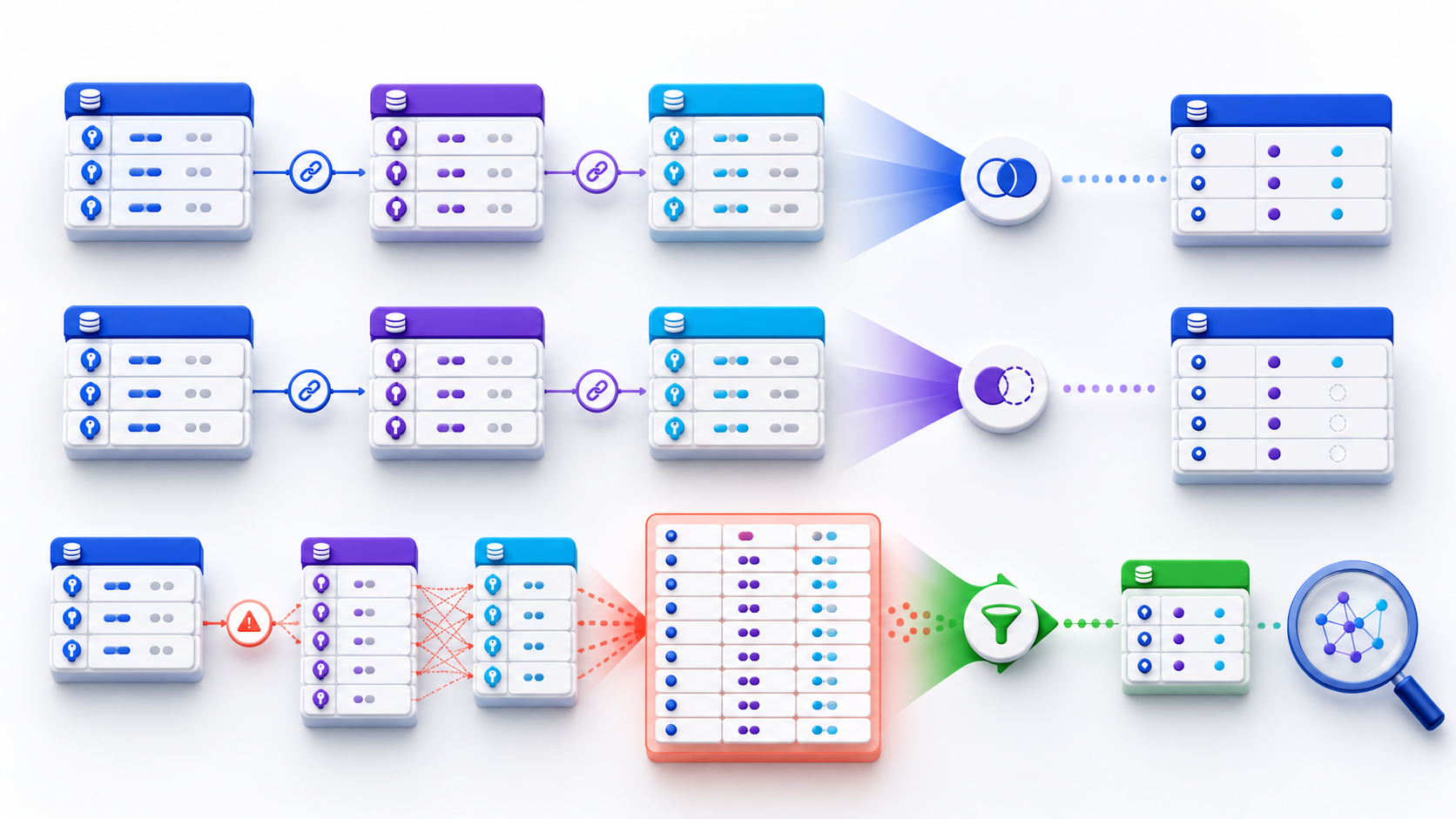
A SQL join returns one row per matching pair. That is join cardinality. If the right side is one-to-many, a “correct” INNER JOIN or LEFT JOIN multiplies the left grain—and DISTINCT only hides it. State what one result row represents, profile key uniqueness, then join. Types still matter: INNER keeps matches, LEFT/RIGHT/FULL also preserve unmatched rows, CROSS returns every pair.
A join adds a relationship, not just columns

The syntax is usually easy; the difficult part is preserving the intended business grain. A join does not merely “add columns.” It can remove rows, create null-extended rows, or multiply one input row into many outputs. Before writing SQL joins, state what one result row should represent and whether unmatched entities belong in the answer.
SELECT o.order_id, o.order_date, c.customer_name
FROM orders o
INNER JOIN customers c
  ON c.customer_id = o.customer_id;
Understand cardinality before joining tables
Uniqueness is data, not join syntax
Cardinality describes how many rows on one side can match a row on the other. Profile keys before you write SQL joins that assume a one-to-one match. A primary-key-to-foreign-key join is commonly many-to-one: many orders can reference one customer, but each order matches at most one customer. Joining from orders to customers normally preserves the order grain. Joining orders to order items is one-to-many and changes the output grain to order item. Neither relationship is inherently bad; problems arise when the query author assumes the original grain still holds.
One key matches at most one row on each side. Row counts usually remain stable when every left key exists.
Multiple facts attach to one dimension row. The fact grain remains intact when the dimension key is unique.
Each parent may produce several outputs. Aggregates calculated after the join must use the new child-level grain.
Several rows on both sides share the join key. Output size can grow multiplicatively and totals are easily inflated.
Uniqueness is data, not syntax. Writing ON a.customer_id = b.customer_id does not prove either column is unique. Check constraints and profile the actual data, including nulls and late-arriving duplicates.
Diagnose duplicate rows created by joins
Every matching pair becomes a row
A join does not randomly create duplicates. This is the most common first failure I see in desk reviews of SQL joins. It returns one row for every pair satisfying the condition. If an order matches three promotions and two support contacts, joining both child tables directly can produce six combinations for that order. A later DISTINCT may hide identical projections, but it does not prove the grain is correct and can discard legitimate differences.
WITH item_totals AS (
  SELECT order_id,
         SUM(quantity * unit_price) AS order_total
  FROM order_items
  GROUP BY order_id
),
payment_totals AS (
  SELECT order_id,
         SUM(amount) AS paid_total
  FROM payments
  GROUP BY order_id
)
SELECT o.order_id, i.order_total, p.paid_total
FROM orders o
LEFT JOIN item_totals i ON i.order_id = o.order_id
LEFT JOIN payment_totals p ON p.order_id = o.order_id;
Each child table is reduced to one row per order before the joins, so the order grain is explicit. Other valid remedies include selecting one child row with a deterministic window rule, using EXISTS when only presence matters, or returning child collections separately. The correct choice depends on what one output row represents.
Choose the join type from the business question
Pick SQL joins from the surviving population
Do not choose a join by habit. The type expresses which population must survive. If a report asks for customers who placed an order, an inner join is appropriate. If it asks for every customer and their latest order when available, the customer table belongs on the preserved side of a left join. If the task is data reconciliation between two systems, a full join may be needed to reveal records missing from either source.
| Join | Rows preserved | Typical question | Main risk |
|---|---|---|---|
INNER JOIN | Matching pairs only | Which orders have a valid customer? | Silent loss of unmatched rows |
LEFT JOIN | All left rows plus matches | Which customers have no orders? | A WHERE filter can remove null-extended rows |
RIGHT JOIN | All right rows plus matches | Same semantics as reversed LEFT JOIN | Direction becomes harder to follow |
FULL JOIN | Matches and both unmatched sides | Which source records disagree? | Null interpretation and reconciliation logic |
CROSS JOIN | Every left-right combination | Generate a complete scenario matrix | N × M row explosion |
The PostgreSQL table-expression documentation defines these join forms and explains that a cross join between N and M rows produces N × M rows. That arithmetic is also the right mental model for accidental multiplication in SQL joins.
Place join conditions and filters deliberately
ON matches; WHERE can rewrite the join
ON defines which pairs match. For outer SQL joins, a predicate in WHERE can drop the unmatched rows you meant to keep. USING is concise when both sides share identically named key columns. NATURAL JOIN infers all same-named columns and is fragile because a schema change can silently alter the relationship. In production analytical SQL, explicit conditions are usually easier to review.
-- Keeps every customer; only completed orders can match
SELECT c.customer_id, o.order_id
FROM customers c
LEFT JOIN orders o
  ON o.customer_id = c.customer_id
 AND o.status = 'completed';

-- Removes customers without a completed order
SELECT c.customer_id, o.order_id
FROM customers c
LEFT JOIN orders o
  ON o.customer_id = c.customer_id
WHERE o.status = 'completed';
The first query preserves every customer because status is part of the match condition. The second evaluates status after the join; null-extended rows fail the predicate, so the result behaves like an inner join for that condition. This difference is central to LEFT JOIN SQL and should be tested with an explicitly unmatched customer before you trust outer SQL joins.
Desk packet: first failures in SQL joins
What I scored on twelve authorized tickets
Label: InfiniSynapse research-desk review of twelve authorized analytics tickets in 2026 H1 (marker DESK-JOIN-20260814A). First-hand notes—not a named-customer case, not a PostgreSQL or Microsoft SLA. I scored the first failing stage after the query parsed.
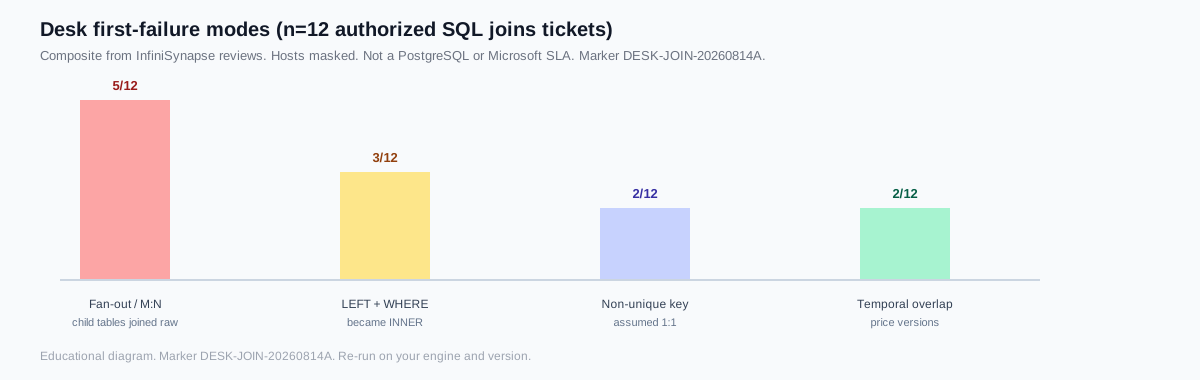
| First failing stage | Tickets | Typical fix |
|---|---|---|
| Fan-out / many-to-many | 5 / 12 | Pre-aggregate or EXISTS before combining children |
| LEFT + WHERE became INNER | 3 / 12 | Move the child predicate into ON |
| Non-unique key assumed 1:1 | 2 / 12 | Profile duplicates; dedupe the dimension |
| Temporal overlap | 2 / 12 | Half-open validity plus a boundary fixture |
Quotable desk assertion (fixture-specific): five of twelve tickets inflated totals because two one-to-many SQL joins sat on the same parent without a prior reduce. Re-run the same evidence standard on your engine and version.
Control complexity in multi-table join queries
Add one relationship at a time
As the graph of SQL joins grows, correctness becomes harder to infer from syntax alone. One join may preserve the grain, the next may expand it, and a third may filter away unmatched rows. Aliases such as a, b, and c make the graph even harder to review. Use role-based aliases, group related logic in named stages, and state the grain after every stage.
- Start with the decision population. Choose the table or subquery that defines which entities can appear.
- Add one relationship at a time. Record expected and actual total rows and distinct business keys.
- Verify the matching key. Check type, nullability, normalization, temporal validity, and uniqueness.
- Declare preservation. Explain why unmatched rows should disappear or remain at each join.
- Reduce child sets early. Aggregate, filter, or rank one-to-many tables before combining them when the final grain is higher.
- Review the entire graph. Inspect CTE dependencies, join count, nested subqueries, windows, and aggregates together.
Use semi, anti, and temporal join patterns precisely
Presence questions should not multiply rows
Some relationship questions should not return columns from both sides. A semi-join asks whether at least one related row exists; an anti-join asks whether none exists. SQL commonly expresses these with EXISTS and NOT EXISTS. They avoid multiplying the preserved entity when several matches exist and communicate that only presence matters—often a safer pattern than extra SQL joins that only need a flag.
SELECT c.customer_id, c.customer_name
FROM customers c
WHERE NOT EXISTS (
  SELECT 1
  FROM orders o
  WHERE o.customer_id = c.customer_id
    AND o.status = 'completed'
);
A left join followed by WHERE child.key IS NULL can express the same anti-relationship, but NOT EXISTS is often clearer and avoids accidental changes when additional child filters are placed in the wrong clause. Be careful with NOT IN: if its subquery can return null, three-valued logic may produce no true comparisons. Confirm the engine's semantics and nullability before using it.
Temporal and range joins match intervals rather than equal keys. For example, an order may need the product price version effective at order_time. The join needs both identity and validity predicates, such as price.valid_from <= order_time and order_time < price.valid_to. Overlapping versions create multiple matches; missing coverage creates unmatched rows. Test boundary timestamps, open-ended intervals, daylight-saving changes, and overlapping effective periods explicitly.
End-to-end: order grain with items, payments, and price history
This is the complex pattern I ask teams to write once before they add more SQL joins: keep the order grain, attach one item total, one payment total, and one effective unit price.
WITH item_totals AS (
  SELECT order_id, SUM(quantity * unit_price) AS item_total
  FROM order_items
  GROUP BY order_id
),
payment_totals AS (
  SELECT order_id, SUM(amount) AS paid_total
  FROM payments
  GROUP BY order_id
)
SELECT o.order_id, i.item_total, p.paid_total, pr.unit_price
FROM orders o
LEFT JOIN item_totals i ON i.order_id = o.order_id
LEFT JOIN payment_totals p ON p.order_id = o.order_id
LEFT JOIN product_prices pr
  ON pr.product_id = o.product_id
 AND pr.valid_from <= o.order_time
 AND o.order_time < pr.valid_to;
If product_prices overlaps, this still fans out. The desk fix is a uniqueness constraint or a window that picks one version, then a fixture that ties order_time to each boundary. That is how I validate production SQL joins that mix children and history.
Separate logical joins from physical execution
Logical SQL joins are not a physical algorithm
SQL states the logical relationship; the database selects physical algorithms such as nested loops, hash joins, or merge joins. A hash join is not automatically good, and a nested loop is not automatically bad. Suitability depends on row counts, selectivity, ordering, memory, indexes, and data distribution. The Microsoft SQL Server join documentation distinguishes logical and physical joins and is a useful reference for plan review.
| Plan signal | Possible meaning | Next check |
|---|---|---|
| Estimated and actual rows diverge | Statistics, correlation, or predicates are misunderstood | Profile key distributions and refresh statistics |
| Large intermediate result | Join expands before selective filtering | Test safe predicate pushdown or pre-aggregation |
| Spill to disk | Hash or sort exceeds available memory | Reduce row width/volume and inspect memory settings |
| Repeated inner scans | Nested loop performs much more work than expected | Check indexes, estimates, and alternative join order |
Performance tuning comes after semantic validation. Fast SQL joins that return multiplied revenue are still wrong. Benchmark with representative parameter values and volume, include cold and warm cache behavior where relevant, and verify that a rewrite returns the same intended rows before comparing runtime.
Validate a SQL join before production
Keep adversarial fixtures as regression tests
Use adversarial fixtures rather than only clean sample data. Test SQL joins the same way you test an API contract. Include an unmatched left row, an unmatched right row, duplicate keys on each side, a null key, a key with different formatting, and a temporally expired relationship. These cases reveal whether the query's preservation and matching rules are explicit.
- Assert expected total rows and distinct business keys.
- Measure unmatched rates from both sides.
- Find keys with more than one match and explain each relationship.
- Compare aggregate totals before and after the join.
- Review selected columns so duplicated facts are not mistaken for new events.
- Run the complete statement through structural review before plan-level tuning.
Inspect the complete SQL join graph
Prepare a sanitized version of the whole statement—not only one JOIN line—so CTEs, subqueries, join count, windows, aggregates, and nesting can be considered together. Use the InfiniSynapse SQL Complexity Checker to identify structural hotspots in SQL joins, then validate semantics and performance in your database.
Commercial association: You do not need the checker to complete the educational diagnosis on this page.
Open SQL Complexity Checker Never paste credentials, secrets, personal data, or sensitive literal values.SQL joins frequently asked questions
What is join cardinality?
Join cardinality is how many rows on one side can match a row on the other. One-to-many changes the output grain: each parent can become several result rows.
Why does a one-to-many SQL join duplicate rows?
A join returns one row for every pair that satisfies the condition. If the child key is not unique, the parent row is copied once per match. Aggregate or rank the child table to one row before you join.
Why does a LEFT JOIN return multiple matches?
LEFT JOIN keeps every left row and still emits one output row per right-side match. Multiple matches duplicate the left row. Reduce the right table first, or the query is working as designed.
What is a SQL join?
SQL joins combine rows from two table expressions according to a matching condition and a preservation rule.
Which SQL join should I use?
Use INNER when only matched entities belong, LEFT when every left entity must remain, FULL for reconciliation, and CROSS only when every combination is intended.
Why do SQL joins create duplicate rows?
Every matching pair becomes an output row, so non-unique keys on both sides multiply the grain.
Does join order matter?
Optimizers often reorder inner joins, but outer joins, lateral references, filters, and nonassociative conditions can make the written structure semantically significant.
How do I check complex SQL joins?
Define grain, profile uniqueness, reconcile row counts after every join, test unmatched and duplicate cases, then inspect the plan.
Official SQL joins documentation
For vendor syntax, use the official docs below. This page is the grain and duplicate-row diagnosis—not a replacement for PostgreSQL or SQL Server documentation.