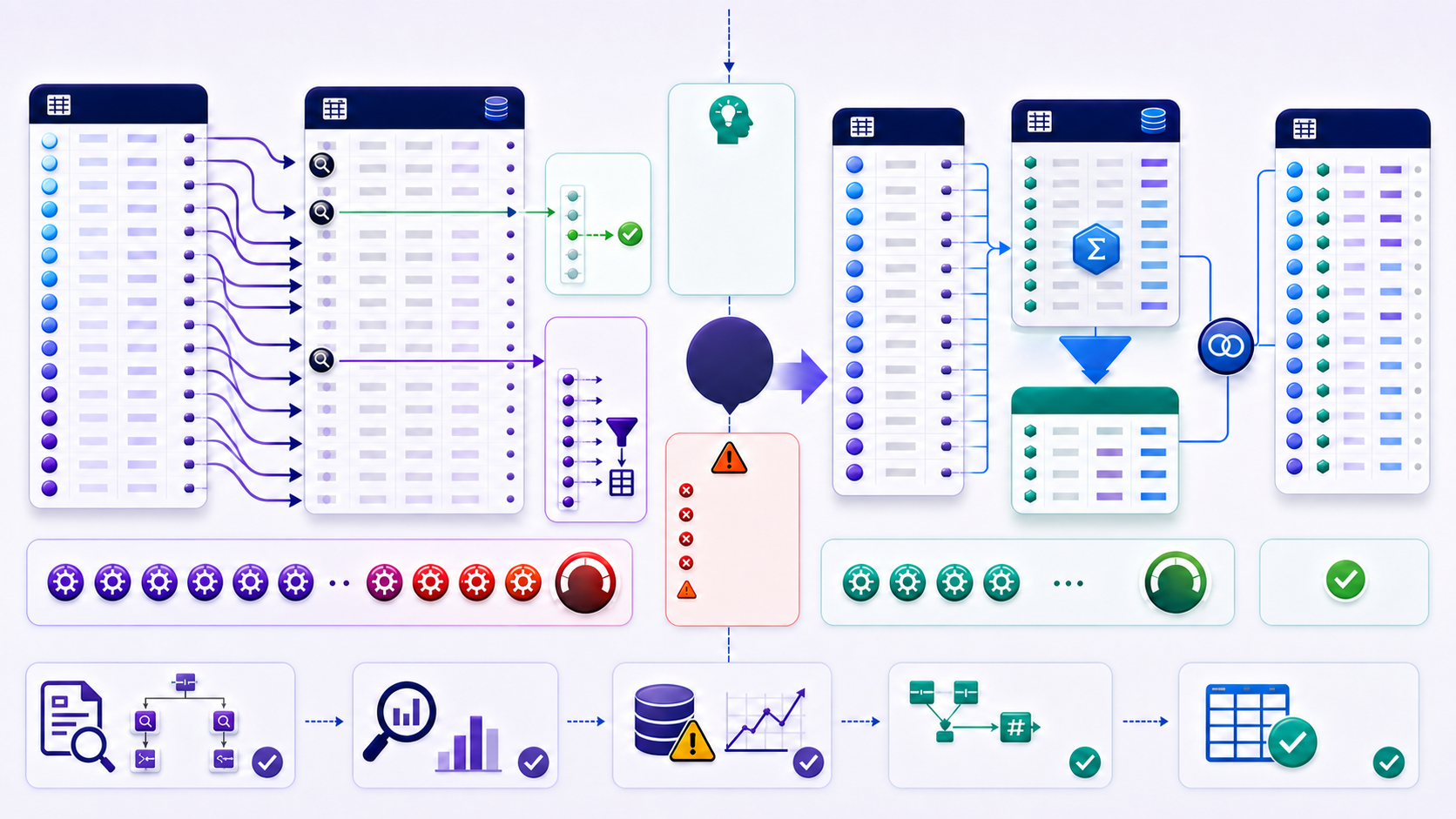
What is a correlated subquery?
A correlated subquery references one or more values from the current row of an outer query. Its logical result therefore depends on that outer row. The database may execute repeated probes or transform the pattern into a join, semi-join, anti-join, aggregate, or another set-based plan.
SELECT e.employee_id, e.salary
FROM employees e
WHERE e.salary > (
  SELECT AVG(x.salary)
  FROM employees x
  WHERE x.department_id = e.department_id
);
The inner average changes with the current employee's department. This is clear SQL, not automatically bad SQL. Risk depends on outer rows, inner work, indexes, statistics, optimizer transformations, and data skew. Inspect actual evidence rather than rejecting correlation by style rule.
How a correlated subquery runs
The logical model has three steps. The optimizer may still turn the pattern into a join, semi-join, or aggregate, so the physical plan is not guaranteed to run the inner query once per outer row.
- Take the current outer row. The outer query supplies the values this row holds, such as
e.department_id. - Run the inner query with those values. The subquery reads the outer row. An independent subquery does not.
- Use the inner result in the outer query. A comparison,
EXISTS, or an assignment consumes that result, then the next outer row repeats the logic.
Who the department-average example keeps
This fixture has four employees. Department 10 averages 60,000. Department 20 averages 80,000. The department-average query in the first section keeps a row only when salary is greater than that department average.
| Employee | Department | Salary | Department average | Result |
|---|---|---|---|---|
| Alice | 10 | 50,000 | 60,000 | Excluded |
| Bob | 10 | 70,000 | 60,000 | Kept |
| Charlie | 20 | 70,000 | 80,000 | Excluded |
| David | 20 | 90,000 | 80,000 | Kept |
Bob and David stay. Alice and Charlie do not. A join rewrite has to keep those same two rows, including the handling of a department with no salaries and a NULL department id.
A window can keep the same row and attach the group average
A window aggregate attaches the department average to every employee and leaves the detail row in place. Filter that average from an outer query, because the window is computed after WHERE in the same SELECT. The comparison with a window function still needs the zero-match, duplicate-key, and NULL checks in the equivalence section. It is not automatically faster than the correlated form.
SELECT employee_id, salary
FROM (
  SELECT employee_id, department_id, salary,
         AVG(salary) OVER (PARTITION BY department_id) AS dept_avg
  FROM employees
) s
WHERE salary > dept_avg;
UPDATE still needs an outer-row reference
A subquery inside UPDATE is correlated only when it reads the row being updated. If it never reads that row, it is an independent subquery, including when it sits in DELETE. Some engines reject a subquery that reads the table being updated; that restriction does not change the correlation test.
UPDATE employees e
SET salary = (
  SELECT AVG(x.salary)
  FROM employees x
  WHERE x.department_id = e.department_id
)
WHERE e.department_id = 10;
Trace every outer reference and its expected cardinality
Aliases make correlation visible. An inner reference to e.department_id reaches outside its own query block, while references to x remain local. Deep nesting can hide which outer level supplies a value. Use distinct aliases and keep the correlation predicate near the inner data source.
Write the return contract too. A correlated scalar subquery must return at most one row per outer row; EXISTS only needs one qualifying row; a correlated aggregate normally returns one value even when no inner rows exist, but that value may be NULL. These shapes have different zero-match behavior.
Use correlated EXISTS for relationship tests
EXISTS asks whether at least one inner row satisfies the correlation and local filters. It does not project child columns or multiply the outer row. An optimizer can often implement it as a semi-join and stop searching after a match. This makes it a natural form for “customers with an open order.”
SELECT c.customer_id
FROM customers c
WHERE NOT EXISTS (
  SELECT 1
  FROM orders o
  WHERE o.customer_id = c.customer_id
    AND o.status = 'open'
);
NOT EXISTS avoids the NULL trap of NOT IN. Still test null and malformed keys, because a null correlation value will not match ordinary equality. Decide whether such outer records belong in “no match,” “invalid key,” or a separate quality category.
Control zero-match behavior in correlated aggregates
A correlated aggregate can compare each entity with its own baseline or return one summary. COUNT(*) over no matching inner rows returns zero; SUM or AVG commonly returns NULL. A left-joined pre-aggregation may reproduce this only if missing groups and COALESCE choices are handled deliberately.
Several correlated scalar subqueries against the same child table can repeat nearly identical work. Calculate all required metrics in one grouped inner stage and join once. Validate that the grouped key is unique and that the outer preservation rule matches the original.
Estimate repeated work before reading the plan
A useful upper-bound model multiplies outer rows by average inner work. Ten thousand outer rows with a selective indexed probe may be cheap; one million outer rows each scanning a large inner range may dominate runtime. Correlation on low-cardinality keys can repeat the same result for many outer rows, suggesting pre-aggregation or caching opportunities.
| Risk factor | Why it matters | Evidence |
|---|---|---|
| Large outer input | More logical probes | Actual outer rows |
| Weak inner access | Each probe reads more | Rows and buffers per loop |
| Skewed key | Some probes explode | Key-frequency percentiles |
Rewrite to aggregate once and join once when semantics allow
WITH department_average AS (
  SELECT department_id, AVG(salary) AS avg_salary
  FROM employees
  GROUP BY department_id
)
SELECT e.employee_id, e.salary
FROM employees e
JOIN department_average d
  ON d.department_id = e.department_id
WHERE e.salary > d.avg_salary;
This computes each department once and exposes a validation boundary. It may still scan and aggregate more inner data than selective probes would, so it is not automatically faster. Compare actual plans with representative predicates. If employees with null or missing departments should remain, join preservation and comparison logic need separate treatment.
Other rewrites include window aggregates, lateral joins, semi-joins, and precomputed summaries. Choose the form that makes grain and work visible, then prove equivalence for zero matches, duplicates, NULL, and boundary values.
Index the correlation path, not the syntax
For repeated probes, the inner index often begins with equality correlation keys, followed by selective local predicates or ordering keys according to the access pattern. A covering index may avoid lookups but increases storage and write cost. Range conditions, functions on keys, implicit casts, and mismatched collations can prevent efficient seeks.
Do not add an index from SQL text alone. Examine existing indexes, workload frequency, selectivity, writes, maintenance, and actual plan evidence. An index that helps one correlated query can overlap another or become unused after decorrelation.
Read loops and rows per loop together
An inner operator showing one row is not cheap if it executes millions of times. Multiply actual rows per loop by loops, then inspect buffers, CPU, elapsed time, spills, remote calls, and cache effects. Compare estimated and actual outer rows because a nested-loop choice based on severe underestimation can fail at scale.
Some engines label a plan as a join even though the SQL is correlated; that indicates transformation, not necessarily full efficiency. Conversely, a nested loop can be optimal for a small selective workload. Benchmark relevant parameter ranges instead of declaring one operator good or bad universally.
Prove correctness before accepting a rewrite
- State the outer grain, correlation key, and inner return contract.
- Test zero, one, and many inner matches plus null keys.
- Compare row counts, distinct outer keys, and metric totals after rewriting.
- Inspect actual loops, rows per loop, reads, estimates, spills, and time.
- Benchmark small, typical, skewed, and large outer populations.
- Verify permissions and remove sensitive literals before external analysis.
- Preserve representative equivalence and performance fixtures.
Diagnose latency that grows with outer rows
Suppose a customer report is fast for one region but times out globally. The plan shows an inner index probe executed once per outer customer. Each probe is quick, yet global outer rows are fifty times larger and one tenant has extreme history. Capture loops and reads by tenant, then compare a grouped-once rewrite. If the rewrite scans all history but removes repeated probes, its advantage appears only beyond a crossover point.
Keep both result equivalence and workload thresholds in the review record. The best plan for interactive single-customer lookup may differ from the best plan for a full export.
Inspect the complete correlated query
Paste a sanitized complete statement into the InfiniSynapse SQL Complexity Checker to review correlation, nesting, repeated structures, joins, aggregation, windows, and filters together. Then confirm repeated work with your actual plan.
Open SQL Complexity CheckerRemove credentials, secrets, personal data, and sensitive literals.Correlated subquery frequently asked questions
A correlated subquery references one or more values from the current row of an outer query, so its logical result depends on that outer row.
Logically it depends on the current outer row. The plan may already be a join, semi-join, or aggregate, so one inner execution per outer row is not guaranteed.
No. Optimizers transform many forms; risk depends on remaining work and scale.
It clearly tests relationship existence without multiplying outer rows.
Often by grouping inner data once and joining on the correlation key, with equivalence tests.
Loops, rows per loop, total reads, time, estimates, spills, and skew.
Official subquery documentation
Build an equivalence proof before replacing correlation
A set-based rewrite changes query structure and can change results even when the happy-path sample agrees. Start with the original outer population and classify keys into no inner match, one match, several matches, null correlation key, malformed key, and high-frequency key. Compare original and rewritten outputs within each class. Use stable business keys and compare both row-level differences and aggregate totals; matching totals can conceal different affected entities.
Preservation is a frequent source of mismatch. A scalar count returns zero for no inner rows, while an inner join to a grouped result removes the outer row entirely. A left join retains it but exposes NULL until converted. A scalar SUM may return NULL, so converting every missing group to zero during the rewrite changes meaning. Write expected zero-match output for every metric before choosing join type and COALESCE behavior.
Performance proof needs more than one benchmark. Measure a single selective outer key, a typical interactive filter, a full export, and a skewed tenant. The correlated plan may win for a tiny selective lookup because it avoids aggregating irrelevant data, while the grouped-once plan may win for a broad report. Record the crossover point, plan shape, reads, CPU, elapsed time, memory, and spill behavior. Parameter-sensitive engines may need separate strategies or plan management.
Keep the original and rewritten queries in a regression harness until the migration is stable. Re-run equivalence after schema constraints, statistics, indexes, or data distributions change. Monitor outer-row count, inner matches per key, unmatched rate, loops, and latency percentiles. A rewrite is complete only when its semantic contract and operating range are both documented, not merely when one execution becomes faster.
Review sensitive row-dependent access
Correlation can also encode row-level eligibility, tenant boundaries, or authorization checks. A performance rewrite must not move those predicates outside their protected scope or aggregate data across tenants before filtering. Include access-policy tests, tenant-crossing adversarial keys, and approved-purpose checks in the equivalence suite. Sanitize plans and SQL before sharing them because literals, object names, and filter values can expose sensitive structure. Correctness includes preserving security boundaries as well as returned rows.
Choose from evidence
Keep correlation when it is clear, correct, and efficient for the operating range. Rewrite it when named stages improve verification or repeated work becomes material. The decision belongs to measured semantics and workload, not a blanket prohibition.