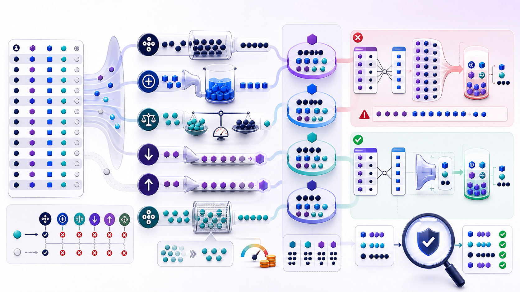
What are SQL aggregate functions?
SQL aggregate functions reduce a set of input rows to one value per group. COUNT measures rows or non-null expressions, SUM adds numeric inputs, AVG divides a non-null sum by a non-null count, and MIN or MAX selects an endpoint. Without GROUP BY, the qualifying input is one group.
SELECT
  customer_id,
  COUNT(*) AS order_count,
  SUM(order_total) AS revenue,
  AVG(order_total) AS average_order
FROM orders
WHERE status = 'completed'
GROUP BY customer_id;
This output has customer grain, but its business meaning still depends on the source: whether refunds are negative orders, whether currency is normalized, whether revisions duplicate an order, and which completion timestamp defines the period. Aggregation does not repair ambiguous data; it compresses whatever rows the query supplies.
Choose COUNT, SUM, AVG, MIN, or MAX by metric definition
Each aggregate answers a different question. COUNT(*) asks how many rows survived. COUNT(expression) asks how many surviving rows have a non-null expression. SUM and AVG require additive or averaging semantics; adding account balances across time is usually wrong, while adding transaction amounts may be valid. MIN and MAX identify endpoints but do not automatically return the other columns from the same row.
| Function | Question | Common trap |
|---|---|---|
COUNT(*) | How many rows? | Rows are not always entities |
SUM(x) | What is the additive total? | Join repeats the measure |
AVG(x) | What is the unweighted mean? | Average of averages |
MIN/MAX | What is the endpoint? | Unrelated projected columns |
Distinguish rows, populated values, and distinct entities
COUNT(*), COUNT(column), and COUNT(DISTINCT column) can all be correct and still produce different numbers. A support-ticket table may have 1,000 rows, 940 non-null assignee IDs, and 47 distinct assignees. Label the metric precisely instead of calling all three “count.” For composite entity identity, some engines accept several expressions in COUNT(DISTINCT ...); others require a derived table of distinct key tuples.
SELECT
  COUNT(*) AS ticket_rows,
  COUNT(assignee_id) AS assigned_rows,
  COUNT(DISTINCT assignee_id) AS active_assignees
FROM tickets
WHERE opened_at >= DATE '2026-07-01';
If the same ticket appears in several snapshot records, row count measures snapshots, not tickets. Define whether the source is event, transaction, version, snapshot, or entity grain before counting. Counting a unique identifier can protect an entity metric, but it may also hide duplicate ingestion that deserves an alert.
Interpret NULL and empty groups explicitly
Most standard aggregates ignore NULL inputs. COUNT(expression) returns zero when no non-null values exist, while SUM, AVG, MIN, and MAX commonly return NULL for an empty or all-null input. That distinction lets SQL preserve “no observed value” instead of inventing zero. Applying COALESCE is a business decision, not merely formatting.
Suppose a left join preserves every store and a store has no sales. COUNT(s.sale_id) correctly returns zero because the non-null sale key has no values. COUNT(*) returns one because the null-extended store row still exists. SUM(s.amount) returns NULL unless converted. Decide whether the consumer needs “no sales recorded,” “zero sales,” or “data unavailable,” because those states may require separate fields.
Compute averages from the correct numerator and denominator
AVG(x) is equivalent in concept to SUM(x) / COUNT(x) over non-null inputs, subject to engine numeric types and precision. It is not equivalent to the average of subgroup averages unless each subgroup has the same weight. To combine daily average order values into a monthly average, retain daily revenue and order count, sum both, then divide.
SELECT
  month_start,
  SUM(revenue) / NULLIF(SUM(order_count), 0) AS average_order
FROM daily_metrics
GROUP BY month_start;
Choose decimal types deliberately to avoid integer division or overflow, and define rounding at the presentation boundary rather than at every intermediate stage. If values carry different exposure, duration, population, or sample weights, model the weighted numerator and denominator explicitly.
Use DISTINCT for metric semantics, not as a join repair
COUNT(DISTINCT customer_id) correctly measures unique customers. SUM(DISTINCT amount) rarely repairs duplicated rows because two legitimate transactions can have the same amount; it removes repeated values, not repeated business records. DISTINCT operations may require hashing or sorting a large state per group, so high-cardinality expressions can be expensive.
When a join duplicates facts, identify the fact key and restore one row per fact before aggregation, or aggregate each relationship at its natural grain before combining. If the desired metric truly counts unique users across several channels, DISTINCT is appropriate, but document identity resolution and whether anonymous, merged, or deleted users change the key.
Prevent joins from multiplying measures before aggregation
The most damaging aggregation bug often occurs before the aggregate. Joining orders to both order items and payments creates one row per item-payment combination. Summing the order total, item amount, or payment amount on that multiplied rowset inflates at least one measure. Draw the relationship graph and label each edge's cardinality before writing the final GROUP BY.
WITH item_totals AS (
  SELECT order_id, SUM(amount) AS item_total
  FROM order_items GROUP BY order_id
), payment_totals AS (
  SELECT order_id, SUM(amount) AS paid_total
  FROM payments GROUP BY order_id
)
SELECT o.order_id, i.item_total, p.paid_total
FROM orders o
LEFT JOIN item_totals i ON i.order_id = o.order_id
LEFT JOIN payment_totals p ON p.order_id = o.order_id;
This keeps each branch at order grain before combining. Validate that each stage truly has one row per order, and decide whether missing branches should remain NULL or become zero. Pre-aggregation is not a universal cure when item and payment detail must be matched by allocation rules; in that case, model the bridge explicitly.
Use conditional aggregation without changing the denominator
Conditional aggregation produces several metrics from one grouped rowset using CASE or an engine's FILTER clause. It is useful for counts by status and related measures, but the ELSE value matters. SUM(CASE WHEN condition THEN 1 ELSE 0 END) counts qualifying rows; COUNT(CASE WHEN condition THEN 1 END) also counts them because false cases become NULL. For averages, returning zero for nonqualifying rows changes the denominator.
Keep the source population shared only when the metrics truly share it. If one metric uses order-created date and another uses payment-settled date, forcing both through one filtered dataset can make one period wrong. Make time basis, status basis, currency basis, and entity grain visible in metric names or documentation.
Review hash, stream, and distinct aggregation costs
A database may use hash aggregation, sort-based or stream aggregation, partial parallel aggregation, and specialized distinct strategies. Large numbers of groups increase state; wide grouping keys increase memory and comparison cost; skew can overload one worker; high-cardinality DISTINCT can spill. An existing useful order may enable streaming, while a filter or pre-aggregation can safely reduce input.
| Plan signal | Likely cause | Check |
|---|---|---|
| Hash spill | More groups or wider state than estimated | Actual groups, width, memory, statistics |
| Expensive sort | Grouping or DISTINCT order | Existing order and unnecessary columns |
| Parallel imbalance | Hot grouping keys | Frequency distribution and partitioning |
Optimization starts after semantic validation. Removing a grouping key changes grain; pushing a filter can change the population; pre-aggregating can remove detail needed for a later condition. Compare actual plans and wall-clock results with representative data, but reconcile every metric before accepting the rewrite.
Validate aggregates with independent controls
- Define the source population, time basis, status basis, currency, and output grain.
- Compare
COUNT(*), non-null counts, distinct entity counts, and duplicate frequencies. - Test empty input, all-null input, zero values, negative values, and extreme numeric values.
- Measure row expansion before aggregation after every one-to-many relationship.
- Reconcile subgroup totals with a direct control total where additivity allows it.
- For averages, preserve and validate numerator, denominator, and weighting rule.
- For MIN or MAX row selection, use a deterministic window or join-back method.
- Inspect actual groups, memory, spills, skew, and estimates in the execution plan.
Trace an inflated metric to the exact relationship
Imagine finance reports that weekly paid revenue exceeds the payment ledger by 18 percent. The reporting query joins orders to items and payments, groups by week, and sums payment amount. Start with three independent controls: payment-ledger total at payment grain, distinct payment count, and order count. Then add the item relationship and measure rows per payment. If a payment appears once for every item on its order, the mechanism is proven; adding SUM(DISTINCT payment_amount) would be unsafe because separate payments can legitimately share an amount.
Repair the model by aggregating items and payments independently to order grain, then join the two controlled stages. Reconcile the repaired weekly total to the ledger and preserve a test order containing several items and several payments. Also monitor maximum items per order, payments per order, and post-join expansion factor. These controls catch the same class of defect when a future relationship—discounts, shipments, refunds, or tax lines—is added to the query.
Inspect the full aggregation pipeline
Paste a sanitized complete statement into the InfiniSynapse SQL Complexity Checker to review joins, grouping layers, DISTINCT operations, windows, subqueries, and repeated structures together. Then reconcile the metric with your source data and actual plan.
Open SQL Complexity CheckerRemove credentials, secrets, personal data, and sensitive literals.SQL aggregate functions frequently asked questions
They summarize a set of rows into one value per group, such as a count, total, average, minimum, or maximum.
COUNT(*) counts rows; COUNT(column) counts rows where the expression is not NULL.
Most expression aggregates ignore NULL inputs, while COUNT(*) still counts the row.
One-to-many or many-to-many matches repeat a measure before the aggregate sees it.
Use it when the metric genuinely depends on unique expression values, not as a generic duplicate repair.