How does a cost savings calculator work?
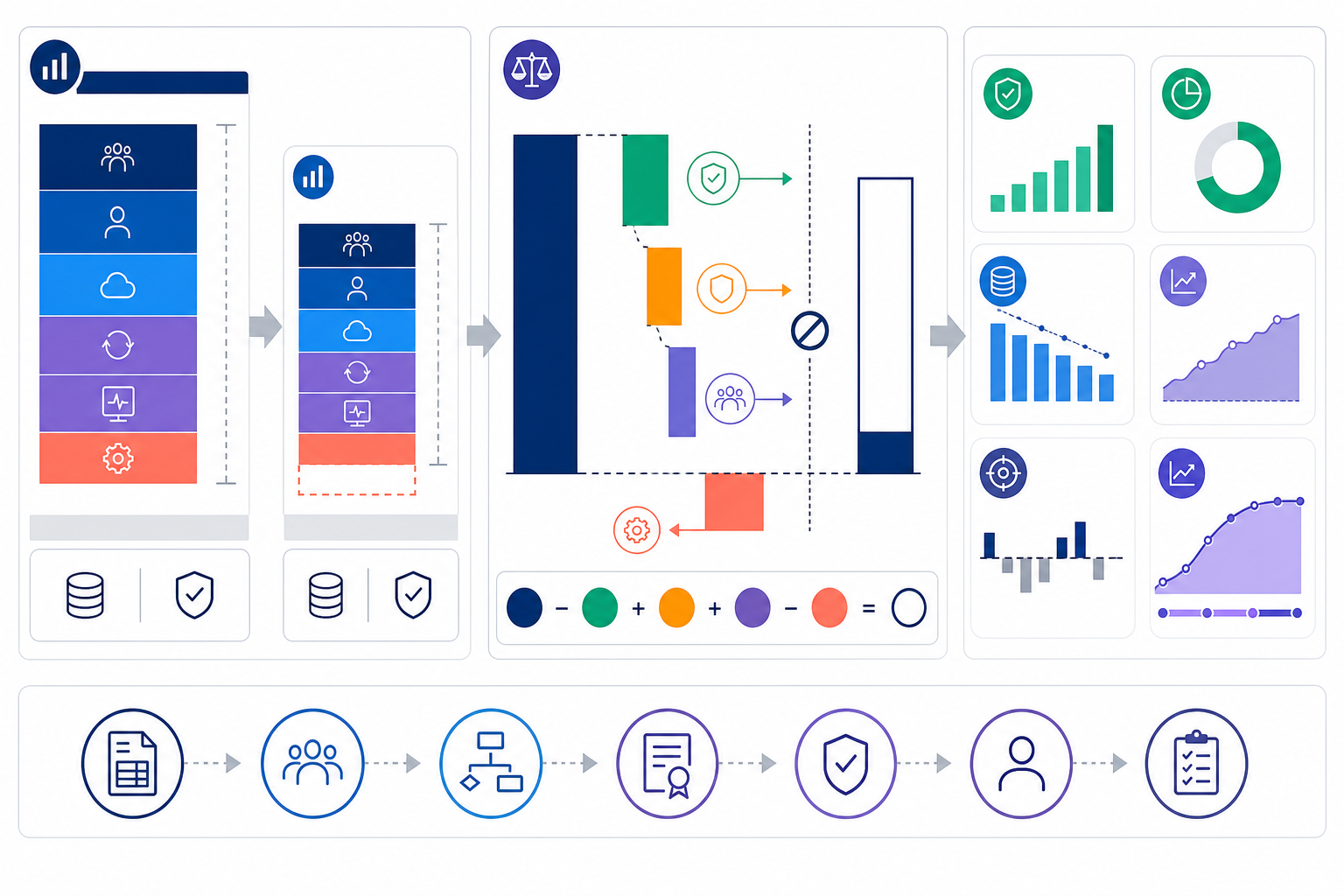
A cost savings calculator subtracts complete post-change cost from the cost of delivering a comparable result under business as usual. In the worked example, annual resource cost falls from $3,960,000 to $2,810,000 for the same 12,000 accepted outputs: a theoretical resource saving of $1,150,000, or 29.0%. Only $310,000 changes cash spend; $840,000 is released internal capacity. After documented reuse, recognized annual capacity value is $588,000, so verified cash plus realized capacity equals $898,000—not the full theoretical difference.
Gross cost savings =
  comparable business-as-usual cost − post-change cost

Savings rate =
  gross cost savings ÷ comparable business-as-usual cost × 100

Net first-year savings =
  first-year realized recurring savings
  − implementation and transition cost
The formula is simple; the comparison is not. A defensible result holds accepted output, task mix, quality, service level, time period, and cost boundary reasonably comparable. It also labels projected, committed, and realized savings separately.
Separate cash savings, cost avoidance, capacity, and economic value
| Category | Recognition rule | Evidence | Financial treatment |
|---|---|---|---|
| Cash saving | Payroll, overtime, contractor, license, cloud, or other actual spend falls. | Ledger, invoice, contract, payroll, or approved budget change | Can enter a cash-flow model when attributable and incremental. |
| Cost avoidance | A credible future cost in the approved baseline no longer occurs. | Approved forecast, trigger, attribution, and revised budget | Report separately from reductions in current spend. |
| Released capacity | Net employee time becomes available after review, rework, support, and exceptions. | Workflow events and comparable time study | Operational measure; not cash by default. |
| Realized capacity value | Released time is demonstrably reused for approved work with an accepted valuation. | Reuse record, accepted output, owner, and finance-approved unit value | Economic value; keep separate from cash unless spend changes. |
| Transfer | Cost moves to another team, vendor, period, or risk owner. | End-to-end cost reconciliation | Not an enterprise saving unless total cost falls. |
A useful calculator keeps these categories in separate rows. Combining them may produce an impressive total that finance cannot reconcile and operations cannot defend. If one mechanism creates two labels, choose one primary claim or document a mutually exclusive split.
Compare the same accepted outcome under the same boundary
“Before” is not automatically business as usual. The valid counterfactual is what the organization would reasonably spend during the comparison period without the change. Adjust for demand growth, committed staffing, contract renewals, price changes, existing efficiency trends, and mandatory controls. Document the adjustment rather than choosing whichever baseline maximizes savings.
Use accepted requests, verified analyses, resolved cases, or another stable unit—not raw attempts.
Segment simple, standard, complex, and high-risk work when their resource needs differ.
Hold acceptance, accuracy, latency, reliability, security, and access requirements constant.
Include the same labor, technology, vendor, facilities, assurance, and overhead rules in both states.
If the after period delivers more work, compare unit cost and build a volume-adjusted baseline. If it delivers lower quality, fewer complex cases, or a slower service level, the raw cost difference is not a saving from efficiency.
Collect the inputs before opening the calculator
| Input | Definition | Preferred source |
|---|---|---|
| Accepted output volume | Units meeting the same acceptance rule in each period | Workflow or service-management system |
| Internal labor hours | Execution, review, correction, exception, support, and management time | Event logs, time study, sampling, payroll owner |
| Fully loaded hourly cost | Wage or salary plus employer benefits and other approved labor costs | Finance or HR; public benchmarks only as a reasonableness check |
| External spend | Contractors, licenses, platforms, cloud, storage, data, support | General ledger, invoice, contract, usage records |
| Implementation cost | Integration, migration, training, redesign, security, evaluation, and transition | Approved work breakdown and actual project costs |
| Realization factor | Share of steady-state savings expected or observed during the period | Rollout schedule, adoption, acceptance, contract timing |
Use a fully loaded labor rate without pretending it is cash
A salary-only rate understates the resources consumed by work. A fully loaded rate may include salary, employer-paid benefits, payroll taxes, paid leave, and allocated overhead according to finance policy. The U.S. Bureau of Labor Statistics Employer Costs for Employee Compensation series measures employer wage and benefit costs per hour worked and can support a broad reasonableness check, but it is not a substitute for your role, geography, level, and accounting policy.
Annual employer labor cost =
  salary + benefits + payroll taxes + other approved labor cost

Productive hours =
  paid hours − leave − holidays − nonproductive time

Fully loaded hourly cost =
  annual employer labor cost ÷ productive hours
The worked example uses an illustrative $80 per hour. Multiplying released hours by this rate estimates resource value; it does not prove a cash saving. Cash changes only when payroll, overtime, contractors, approved hiring, or another ledger item changes.
Step 1: build the comparable annual baseline cost
The hypothetical analytics workflow delivers 12,000 accepted outputs per year. Baseline internal labor is 36,000 hours, or 3.0 hours per accepted output after execution, review, rework, exceptions, and support. Contractors and technology are assigned to the same workflow boundary.
| Baseline resource | Input | Calculation | Annual cost |
|---|---|---|---|
| Internal labor | 36,000 hours at $80 | 36,000 × $80 | $2,880,000 |
| Contractors | Approved annual invoices | Ledger total | $480,000 |
| Technology and cloud | Licenses, compute, storage, data, support | Allocated invoices and usage | $600,000 |
| Comparable baseline total | 12,000 accepted outputs | — | $3,960,000 |
The baseline should reconcile with finance and operations. If the ledger is $3.96 million but the workflow allocation totals $3.5 million, resolve or disclose the $460,000 difference before claiming savings.
Step 2: build the complete post-change operating cost
The AI-assisted process delivers the same 12,000 accepted outputs under the same quality and service rules. Internal labor falls only after counting prompt or query preparation, human review, corrections, exceptions, monitoring, support, and governance. New assurance cost appears explicitly rather than disappearing inside a productivity claim.
| Post-change resource | Input | Calculation | Annual cost |
|---|---|---|---|
| Internal labor | 25,500 hours at $80 | 25,500 × $80 | $2,040,000 |
| Contractors | Reduced approved invoices | Ledger total | $160,000 |
| Technology and cloud | Retained and new platform usage | Allocated invoices and usage | $520,000 |
| Monitoring and governance | Evaluation, controls, review cadence, support | Approved operating plan | $90,000 |
| Post-change total | 12,000 accepted outputs | — | $2,810,000 |
Step 3: calculate the gross savings amount and savings rate
Gross resource savings =
  $3,960,000 − $2,810,000
  = $1,150,000

Savings rate =
  $1,150,000 ÷ $3,960,000 × 100
  = 29.0%

Resource cost per accepted output:
  before = $3,960,000 ÷ 12,000 = $330.00
  after  = $2,810,000 ÷ 12,000 = $234.17
  unit savings = $95.83
This 29.0% is a steady-state resource-cost reduction, not yet a cash saving, first-year saving, or ROI. The calculation says the comparable operating model uses $1.15 million less annual resource value. The next steps classify what changes the ledger, what releases capacity, and what is actually realized.
Step 4: bridge the theoretical difference to cash and capacity
| Change | Before | After | Difference | Classification |
|---|---|---|---|---|
| Internal labor resource | $2,880,000 | $2,040,000 | $840,000 | Released capacity unless payroll or hiring changes |
| Contractor invoices | $480,000 | $160,000 | $320,000 | Verified cash saving after invoice reconciliation |
| Technology and cloud | $600,000 | $520,000 | $80,000 | Cash saving if allocation and usage are comparable |
| New monitoring and governance | $0 | $90,000 | −$90,000 | New recurring cash cost |
| Total bridge | $3,960,000 | $2,810,000 | $1,150,000 | $310,000 cash + $840,000 capacity |
Cash saving =
  contractor reduction + technology reduction − new assurance cost

= $320,000 + $80,000 − $90,000
= $310,000
The $310,000 should be reconciled to actual contractor, platform, cloud, and governance transactions. If the after-state platform invoice is lower only because usage temporarily fell, the analyst must separate the intervention effect from demand.
Step 5: value only the capacity that is demonstrably reused
Internal labor falls from 36,000 to 25,500 hours, releasing 10,500 hours. At $80 per hour, theoretical capacity value is $840,000. The team documents that 70% of released time—7,350 hours—is reused for approved backlog and recurring decision support. The remaining 3,150 hours are visible but not monetized.
Released hours = 36,000 − 25,500 = 10,500

Documented reused hours = 10,500 × 70% = 7,350

Realized capacity value = 7,350 × $80 = $588,000

Verified cash + realized capacity value =
  $310,000 + $588,000
  = $898,000
The $898,000 is an economic-value view containing two clearly labeled components. It must not be reported as $898,000 of cash savings. The theoretical $252,000 capacity difference not linked to reuse remains an operational opportunity, not recognized value.
Step 6: calculate a savings realization rate
A realization rate shows how much of the theoretically available resource improvement becomes verified cash or approved reused capacity. It is useful only when numerator and denominator use the same categories.
Economic realization rate =
  verified cash savings + realized capacity value
  ÷ theoretical resource savings

= $898,000 ÷ $1,150,000
= 78.1%
Do not compare cash-only realized savings with a denominator that includes all capacity value and then call the result poor execution. Use a cash realization rate for cash forecasts, a capacity reuse rate for hours, and a combined economic realization rate only when the valuation rule is approved.
Step 7: subtract implementation cost from phased first-year savings
Steady-state savings rarely begin on the first day. The example uses a 65% first-year realization factor to reflect a pilot, phased rollout, adoption, contract timing, and learning. One-time implementation and transition cost is $280,000.
| First-year view | Steady-state annual amount | Realization factor | First-year realized amount |
|---|---|---|---|
| Verified cash savings | $310,000 | 65% | $201,500 |
| Realized capacity value | $588,000 | 65% | $382,200 |
| Combined economic value | $898,000 | 65% | $583,700 |
| Implementation and transition | — | One-time | −$280,000 |
Net first-year cash impact =
  $201,500 − $280,000
  = −$78,500

Net first-year economic value =
  $583,700 − $280,000
  = $303,700
Both answers can be correct because they answer different questions. The cash view says the project uses $78,500 more cash than it releases in year one. The economic view says it creates $303,700 of net value after recognizing documented capacity reuse. Present them side by side; never use economic value to imply that the cash budget has already improved.
Normalize cost savings when output volume changes
If accepted output rises after implementation, comparing total spend alone can understate efficiency. If output falls, it can overstate savings. Build the business-as-usual cost for the after-period volume using stable unit-cost drivers, then adjust for price, task mix, quality, and scale effects.
Baseline unit cost =
  baseline cost ÷ baseline accepted units

Volume-adjusted BAU cost =
  expected baseline cost at after-period volume,
  adjusted for price, task mix, service, and scale

Volume-adjusted savings =
  volume-adjusted BAU cost − actual post-change cost
A simple linear estimate would multiply $330 by the after-period accepted output count. That is acceptable only if marginal cost, task mix, and capacity constraints are stable. Fixed contracts, tiered cloud rates, queueing, scarce reviewer capacity, and mixed complexity can make a nonlinear model more appropriate.
Separate recurring savings, one-time savings, and one-time costs
| Timing class | Examples | Modeling rule |
|---|---|---|
| Recurring saving | Reduced contractor retainer, license seats, compute consumption, overtime | Model each period while the mechanism persists; reflect price and volume changes. |
| One-time saving | Refund, avoided migration event, asset sale | Record once in the period realized. |
| Recurring new cost | Platform usage, evaluation, monitoring, support, security controls | Subtract from recurring savings for the same period. |
| One-time new cost | Integration, migration, training, data cleanup, transition, decommissioning | Subtract in the period incurred; do not spread invisibly across recurring savings. |
For a multi-year decision, place each effect in a cash-flow schedule and use the appropriate discounting method. The worked ROI example shows how recurring savings, costs, NPV, and payback fit together and should be used after this savings bridge is reconciled.
Calculate break-even volume, hours, or realization
A break-even calculation identifies the minimum operating result required to cover implementation cost or recurring fixed cost. Choose the driver linked to the mechanism: accepted outputs, avoided contractor hours, reused internal hours, or unit-cost reduction.
Break-even accepted outputs =
  fixed implementation cost ÷ net recurring saving per accepted output

Break-even reused hours =
  fixed implementation cost ÷ approved value per reused hour

Required first-year realization factor =
  implementation cost ÷ steady-state annual economic value

For this example:
  $280,000 ÷ $898,000 = 31.2%
The project needs 31.2% of steady-state combined economic value during year one to offset the $280,000 implementation cost. This does not mean 31.2% cash realization is enough: the cash-only requirement would be $280,000 ÷ $310,000, or 90.3%, and even that assumes the recognized cash saving is available during the year.
Reconcile projected, committed, and realized savings
| Stage | Meaning | Minimum evidence |
|---|---|---|
| Opportunity | Technically possible difference before feasibility and effort | Diagnostic data and mechanism |
| Projected | Modeled saving under stated adoption, timing, cost, and quality assumptions | Approved baseline, model, assumptions, scenarios |
| Committed | Owner has approved an action that should change spend or capacity | Contract notice, budget action, rollout plan, accountable owner |
| Realized | Post-change evidence confirms the effect relative to the approved counterfactual | Ledger, usage, payroll, accepted output, quality, attribution, reconciliation |
Use a variance bridge rather than overwriting the forecast. Explain differences caused by demand, price, task mix, adoption, acceptance, review effort, contract timing, implementation delay, and model error. FinOps forecasting guidance treats forecasts as agreed expectations that should be updated and managed with accountable owners, while usage optimization guidance emphasizes tracking recommendations through action and measuring actual impact against estimates.
Stress-test the savings estimate with causal scenarios
Do not apply an arbitrary plus-or-minus percentage to every input. The U.S. Government Accountability Office cost guide emphasizes linking sensitivity tests to technical baseline parameters, assumptions, and model inputs. Build scenarios around mechanisms that can actually change.
| Scenario | Causal change | Savings effect | Evidence to monitor |
|---|---|---|---|
| Slow adoption | Fewer eligible tasks use the new workflow. | Lower labor release and delayed contractor reduction | Eligible exposure, active use, contract timing |
| Review expansion | Quality risk requires more human review and correction. | Lower net recovered hours; higher operating cost | Review minutes, overrides, escaped defects |
| Usage-price growth | Token, compute, storage, or data use rises faster than output. | Technology savings shrink or become a new cost | Cost per accepted output and rate schedule |
| Demand growth | Output rises beyond the original capacity range. | Total spend may rise while unit cost still improves. | Accepted volume, task mix, marginal cost |
| No capacity reuse | Released hours remain idle or are absorbed invisibly. | Cash view remains; capacity value falls toward zero | Named reused work, accepted output, owner |
HM Treasury's Green Book also recommends explicit business-as-usual assumptions, optimism-bias adjustments informed by historical forecast errors, sensitivity analysis, and switching values. Use your own historical forecast error where available rather than borrowing a generic uplift without context.
Build an evidence register that can survive review
| Record | Required fields | Review owner |
|---|---|---|
| Baseline | Period, population, output, task mix, quality, costs, adjustments, source | Operations and finance |
| Savings item | Unique ID, mechanism, category, formula, timing, owner, overlap check | Benefit owner and finance |
| Cost item | Work breakdown, one-time/recurring, allocation, invoice or labor source | Project and cost owner |
| Operational result | Eligible exposure, accepted output, net hours, review, rework, exceptions | Process and quality owner |
| Reconciliation | Forecast, actual, variance driver, correction, approval, version | Finance and decision owner |
GAO's cost estimating guide describes reliable estimates as comprehensive, well documented, accurate, and credible, with technical baselines, assumptions, data, sensitivity and risk analysis, documentation, presentation, and updates using actual cost. These disciplines scale down to an internal savings case even when the project is much smaller than a major public acquisition.
Protect quality, reliability, security, and risk while saving cost
A lower cost is not a saving if the workflow shifts correction to users, increases decision error, weakens data controls, or creates future remediation. Define guardrails before the pilot and price the resources required to maintain them.
| Guardrail | Measure | Savings-model response |
|---|---|---|
| Acceptance and correctness | First-pass acceptance, severity-weighted defects, reviewer overrides | Add review/rework cost; stop recognition if standards fail. |
| Service | Cycle time, queue, coverage, escalation, availability | Do not claim savings from slower or inaccessible service. |
| Data and security | Approved access, retention, incidents, sensitive-data handling | Include control and residual-risk cost; use a nonfinancial stop rule. |
| Resilience and dependency | Fallback, vendor availability, migration effort, price exposure | Model recurring assurance, exit, and disruption scenarios. |
Map savings inputs into the ROI Calculator
Use this page to reconcile the savings bridge first. Then enter only approved, non-overlapping benefits and complete costs into the ROI Calculator. A calculator applies formulas consistently; it cannot determine whether a saved hour is cash, whether a baseline is fair, or whether quality remained acceptable.
| Prepared input | Example value | Use in the next model |
|---|---|---|
| One-time implementation cost | $280,000 | Initial investment or year-zero cost |
| Verified recurring cash saving | $310,000 | Cash benefit, phased by actual timing |
| Approved realized capacity value | $588,000 | Separate economic benefit when the reuse rule is approved |
| First-year realization factor | 65% | Timing/adoption adjustment, not a blanket confidence score |
| Recurring platform and assurance cost | Already netted in the $310,000 cash bridge | Do not subtract twice; preserve the supporting schedule. |
Turn verified savings into a complete investment view
Bring your reconciled baseline, annual cash savings, approved capacity value, implementation cost, recurring cost, timing, and scenarios. Treat the output as a planning estimate and validate it with actual results.
Open ROI CalculatorUse a ten-step cost savings calculation workflow
- Write the decision and owner.Name the intervention, alternative, deadline, cost owner, benefit owner, and approval condition.
- Define accepted output.Specify the unit, quality threshold, service level, task mix, and exclusions.
- Build business as usual.Forecast what cost and performance would be without the intervention.
- Collect full cost.Include labor, vendors, technology, assurance, support, overhead, implementation, and transition.
- Normalize the comparison.Adjust volume, task mix, price, quality, service, and timing so the states are comparable.
- Calculate gross difference.Show savings amount, baseline-denominator savings rate, and unit-cost change.
- Classify each effect.Separate cash, avoidance, capacity, realized value, transfer, recurring, and one-time effects.
- Apply timing and realization.Use rollout, adoption, contract, acceptance, and reuse evidence rather than assuming immediate steady state.
- Stress-test and set guardrails.Test causal uncertainty and define quality, security, reliability, and stop conditions.
- Reconcile actuals and revise.Compare the approved forecast with ledger and operational results; explain variance and preserve versions.
Avoid these common cost savings calculator errors
| Error | Why it fails | Correction |
|---|---|---|
| Using last year as an unadjusted baseline | Demand, price, task mix, and committed change may differ. | Build an approved BAU counterfactual. |
| Dividing savings by after cost | It answers a different ratio and overstates the standard savings rate. | Use comparable baseline cost as the denominator. |
| Treating gross hours as savings | Review, correction, exception, support, and adoption disappear. | Measure net end-to-end hours for accepted work. |
| Calling capacity cash | The ledger may not change. | Separate cash and prove capacity reuse before valuation. |
| Omitting new operating cost | Platform use, monitoring, evaluation, governance, and support are real. | Use complete incremental cost. |
| Assuming immediate steady state | Pilot, rollout, contract, and learning delays inflate year-one savings. | Model monthly or quarterly realization. |
| Double counting one mechanism | The same hours appear as cash, avoided hiring, and output value. | Use a unique benefit register and overlap review. |
Frequently asked questions about cost savings calculations
How do you calculate cost savings?
Subtract the complete post-change cost from the comparable business-as-usual cost. Divide that difference by business-as-usual cost for the savings rate, then separate cash, avoidance, and capacity effects.
What is the cost savings percentage formula?
Cost savings percentage equals comparable baseline cost minus post-change cost, divided by comparable baseline cost, multiplied by 100.
Should implementation cost be included in cost savings?
Report recurring savings separately, then subtract one-time implementation and transition costs when calculating first-year or cumulative net savings.
Are employee hours saved a cash saving?
Not unless payroll, overtime, contractors, or approved hiring spend changes. Otherwise, net saved hours are capacity and should be valued only when documented reuse creates an approved outcome.
How do you compare costs when output volume changes?
Compare cost per accepted unit and create a business-as-usual cost for the after-period volume, adjusting for task mix, prices, quality, and service levels.
What is the difference between projected and realized savings?
Projected savings are model estimates. Realized savings are supported by post-change invoices, payroll, contracts, usage, accepted output, and finance reconciliation against the approved baseline.
Methods and primary sources
The figures and calculations are original hypothetical examples. The following primary or authoritative sources support the cost-estimating, labor-cost, business-as-usual, sensitivity, forecasting, optimization, and unit-economics methods.
- U.S. Government Accountability Office, Cost Estimating and Assessment Guide (GAO-20-195G)
- HM Treasury, The Green Book 2026
- FinOps Foundation, Forecasting capability
- FinOps Foundation, Usage Optimization capability
- FinOps Foundation, Unit Economics capability
Method note: the worked example uses a comparable 12,000 accepted outputs, an illustrative $80 fully loaded hourly resource cost, a 70% documented capacity-reuse rate, a 65% first-year realization factor, and $280,000 one-time implementation cost. Cash and capacity are never combined without labels. No figure is a product-performance claim or guaranteed saving.