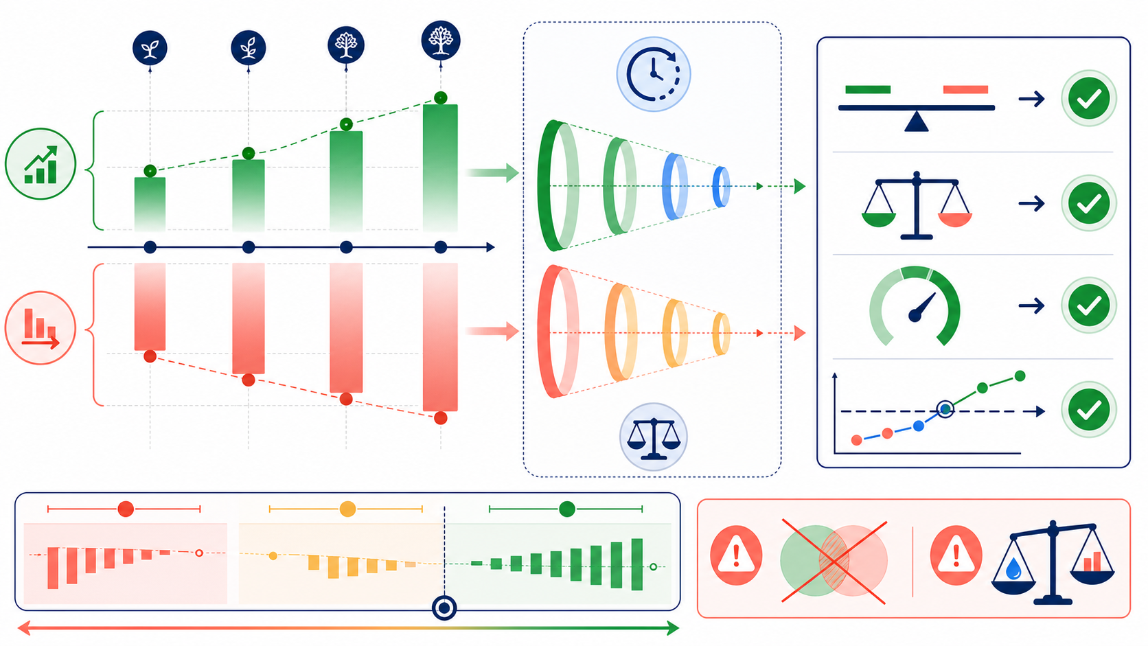
What is the cost benefit analysis formula?
Discount every incremental benefit and cost to present value, then calculate net present value as benefits minus costs and the benefit-cost ratio as benefits divided by costs. For an AI project, use only realized, attributable benefits; include implementation, integration, adoption, review, rework, risk, and operating costs; and test how uncertainty changes the result.
Present value of benefits (PVB) =
  Σ [Benefit at time t ÷ (1 + discount rate)^t]

Present value of costs (PVC) =
  Σ [Cost at time t ÷ (1 + discount rate)^t]

Net present value (NPV) = PVB − PVC

Benefit-cost ratio (BCR) = PVB ÷ PVC

Return on investment (ROI) =
  (PVB − PVC) ÷ PVC × 100%
The cost benefit analysis formula is simple; the difficult work is defining a credible “with-project” change against business as usual, assigning costs and benefits to the correct period, avoiding double counting, selecting consistent units and discount rates, and preserving non-monetized impacts beside the summary metrics.
Choose the metric that answers the decision
| Metric | Formula | Question answered | Limit |
|---|---|---|---|
| NPV | PVB − PVC | How much net present value does the option create? | Scale favors larger projects; uncertainty remains hidden without ranges. |
| BCR | PVB ÷ PVC | How much discounted benefit is generated per unit of cost? | Sensitive to what is placed in the numerator and denominator. |
| ROI | (PVB − PVC) ÷ PVC | What net return is generated as a percentage of cost? | Definitions vary; state whether inputs are discounted and what costs are included. |
| Discounted payback | First period where cumulative discounted net benefit ≥ 0 | How long until the investment recovers its cost? | Ignores value after the crossing point when used alone. |
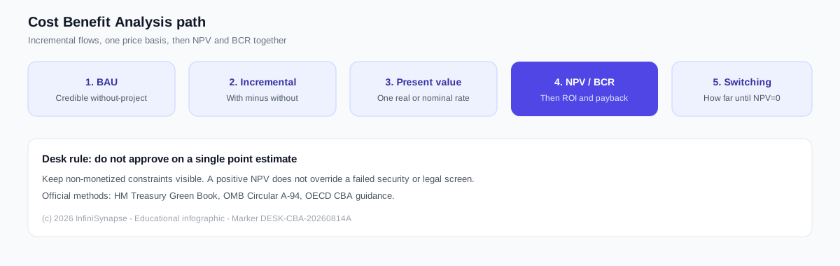
In the cost benefit analysis formula, use NPV and BCR together. With identical discounted inputs, ROI equals BCR minus one, expressed as a percentage: a BCR of 1.70 corresponds to approximately 70% ROI. Pair the result with the ROI example. Payback adds a liquidity and timing view but should not replace lifetime value. No single metric determines strategic fit, operational feasibility, legal permission, or acceptable risk.
Calculate incremental value against business as usual
The cost benefit analysis formula compares options, not a project against zero. Define business as usual as the credible future without the proposed investment, including existing contracts, expected demand growth, required maintenance, known hiring, and planned process changes. Then calculate only the difference caused by each option.
Incremental benefit at time t =
  outcome with project at t − outcome under business as usual at t

Incremental cost at time t =
  cost with project at t − cost under business as usual at t
For example, if analysis demand would rise 15% without AI and the team would already add two contractors, avoided contractor cost may be incremental. If a contract was ending regardless of the project, its removal is not an AI benefit. Record the owner and evidence for every business-as-usual assumption.
Desk lab: two sanitized cost benefit analysis formula packets
These notes are sanitized composites from InfiniSynapse engineer reviews of authorized AI-project packets in 2026 H1 (marker DESK-CBA-20260814A). Hosts and dollar figures are masked. They are first-hand reading notes, not audited customer SLAs. Re-run on your approved path. Independence: educational sections are separate from the commercial ROI calculator CTA.
Case A: cost benefit analysis formula approved hours that were never reused
A team counted every analyst minute saved as cash. The cost benefit analysis formula showed BCR 1.9. Review logs showed recovered time sat idle. After applying an evidenced reuse rate of 40%, NPV fell below zero. The fix was one value route: reused capacity only.
Case B: cost benefit analysis formula mixed a real rate with nominal licenses
Licenses were inflated 4% a year while the discount rate was a real 8% with inflation already stripped. Switching to a consistent nominal pair cut BCR from 1.6 to 1.21. Official HM Treasury discounting guidance matches this order.
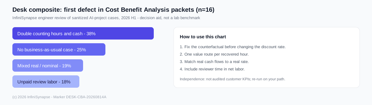
We reviewed 16 sanitized cost benefit analysis formula packets. First defect share: double counting 38%, missing business-as-usual 25%, mixed real/nominal 19%, unpaid review labor 18%. Percentages are decision aids, not vendor performance claims.
Include the complete cost benefit analysis formula boundary
| Category | AI data-project examples | Evidence |
|---|---|---|
| Initial costs | Procurement, integration, security review, migration, training, workflow design | Quotes, work plans, fully loaded labor, contingency |
| Recurring costs | Licenses, usage, hosting, monitoring, support, evaluation, governance | Contracts, rate cards, architecture estimates, owner forecasts |
| Transition costs | Dual running, temporary throughput loss, correction, retraining, decommissioning | Pilot observations, rollout plan, historical transitions |
| Operational benefits | Accepted capacity, faster cycle time, lower rework, fewer data incidents | Controlled comparison, workflow logs, review records |
| Financial benefits | Avoided contractor spend, deferred hiring, incremental serviced demand | Approved budgets, invoices, demand and unit-value records |
| Risk impacts | Error, privacy, security, model failure, concentration, lock-in | Event probability, impact range, control effectiveness, residual risk |
The cost benefit analysis formula uses opportunity cost for internal labor: time spent implementing the project cannot simultaneously deliver another priority. Keep sunk costs—past spending that cannot change—outside the forward decision, while still recording them for governance or lessons learned. For the lifecycle cost boundary, see total cost of ownership.
Discount future costs and benefits consistently
The cost benefit analysis formula discounts values occurring in different years to a common present-value basis. A future value is divided by one plus the discount rate raised to the period number. Year 0 is not discounted. Use the organization’s approved rate and valuation policy; do not copy a public-sector social discount rate into a private investment model without confirming that it answers the same question. HM Treasury discounting guidance and OMB Circular A-94 both require a consistent real or nominal pair.
Present value at time t =
  future amount at t ÷ (1 + discount rate)^t

Discount factor at time t =
  1 ÷ (1 + discount rate)^t
Real model
Express values in constant purchasing power with general inflation removed, then use a real discount rate. Model material relative price changes separately.
Nominal model
Include expected inflation in each cash flow and use a nominal discount rate. Keep the inflation basis consistent across benefits and costs.
Do not add inflation to a real discount rate and then apply it to nominal cash flows without a consistent conversion. State the currency, price year, nominal or real basis, tax treatment, discount rate, timing convention, and horizon at the top of the model.
Apply six cost benefit analysis formula rules before calculating BCR or NPV
- Use incremental flows. Subtract the business-as-usual outcome from every option.
- Use one price basis. Keep all values real or all values nominal with a matching rate.
- Assign the correct period. Record when resources are consumed and benefits are realized, not when a slide predicts them.
- Use mutually exclusive value routes. Do not count the same recovered hour as avoided cost, added output, and strategic capacity.
- Include negative effects. Model correction, downtime, incidents, transition loss, and residual risk.
- Keep an evidence register. Attach source, owner, method, date, confidence, and refresh rule to each input.
Calculate a three-year cost benefit analysis formula example
This hypothetical cost benefit analysis formula example evaluates an AI-assisted data-analysis workflow over three years using an 8% discount rate. Year 0 includes implementation, integration, and training. Annual benefits combine mutually exclusive, verified routes: avoided external analysis, realized value from reused capacity, and lower rework. All figures are illustrative and rounded.
| Year | Benefits | Costs | Discount factor | PV benefits | PV costs |
|---|---|---|---|---|---|
| 0 | $0 | $140,000 | 1.0000 | $0 | $140,000 |
| 1 | $140,000 | $48,000 | 0.9259 | $129,630 | $44,444 |
| 2 | $184,000 | $50,000 | 0.8573 | $157,750 | $42,867 |
| 3 | $213,000 | $52,000 | 0.7938 | $169,086 | $41,280 |
| Total | $537,000 | $290,000 | — | $456,466 | $268,591 |
The base case has positive NPV, BCR above 1, and discounted payback during year 2. That is not an automatic approval. Review whether the benefit evidence is attributable, whether the option meets nonfinancial constraints, whether a lower-cost option creates better value, and whether downside scenarios remain acceptable. Reproduce the arithmetic from the desk CSV (marker DESK-CBA-20260814A).
Interactive desk chart. Toggle a scenario to see NPV and BCR from the same cost benefit analysis formula. Figures are first-party and illustrative — not a third-party lab result.
Base case: PVB $456,466 · PVC $268,591 · NPV $187,876 · BCR 1.70. Same inputs as the table above.

Calculate discounted payback with uneven cash flows
The cost benefit analysis formula should not divide initial cost by an average annual benefit when cash flows vary. See also the payback period guide. Accumulate discounted net benefits period by period. In the example, the unrecovered balance after year 1 is $54,815. Year 2 contributes $114,883 of discounted net benefit, so interpolation gives approximately 1 + 54,815 ÷ 114,883 = 1.48 years.
Discounted net flow at time t =
  (benefit at t − cost at t) ÷ (1 + rate)^t

Payback =
  full periods before crossing
  + unrecovered balance before crossing
    ÷ discounted net flow in crossing period
Interpolation assumes the crossing-period flow arrives evenly. If benefits arrive at a known date—such as annual contract avoidance—use monthly or quarterly periods instead. State whether the reported payback is simple or discounted because they answer different questions.
Prevent double counting in the cost benefit analysis formula
| Potential overlap | Why it duplicates value | Control |
|---|---|---|
| Hours saved + salary savings | Salary continues unless spend or staffing changes. | Classify hours as capacity; count cash only when demonstrably avoided. |
| Avoided hiring + capacity value | Both may represent the same demand coverage. | Choose one route for each workload unit. |
| Faster decisions + full revenue uplift | Revenue may already embody the timing benefit. | Map the causal chain and monetize one attributable endpoint. |
| Fewer errors + avoided incident loss | The same reduced events can appear twice. | Use event count × probability-adjusted impact once. |
| Time saved by analyst + reviewer | AI may move rather than remove labor. | Measure net labor across the end-to-end workflow. |
Create a cost benefit analysis formula value ledger with one row per outcome, a unique identifier, causal mechanism, baseline, formula, owner, and overlap group. If two rows share the same overlap group, explain why both remain or remove one.
Test sensitivity, scenarios, and switching values
A point estimate hides decision risk. After you run the cost benefit analysis formula, use one-way sensitivity to identify influential inputs, coherent scenarios to show combinations of conditions, and switching values to show how far an assumption can move before the decision rule changes.
| Scenario | Benefit assumption | Cost assumption | NPV | BCR |
|---|---|---|---|---|
| Downside | 20% below base | 10% above base | $69,723 | 1.24 |
| Base | Observed planning case | Current estimate | $187,876 | 1.70 |
| Upside | 15% above base | Current estimate | $256,346 | 1.95 |
With costs unchanged, the example reaches BCR 1 when realized benefits fall to about 58.8% of the base forecast. In other words, benefits can fall by roughly 41.2% before NPV reaches zero. This is a switching value, not a probability. Pair it with evidence about how plausible such a shortfall is.
Do not create a “downside” scenario by changing only one convenient variable. Link adoption, productivity, quality, demand, capacity reuse, and support cost in ways that can occur together. Preserve the formula and source behind every scenario value.
Value AI benefits from observed operational evidence
Eligible annual tasks =
  total annual tasks × eligible share

AI-exposed tasks =
  eligible tasks × observed adoption

Net hours recovered =
  exposed tasks ×
  (baseline labor − assisted labor − review − rework) ÷ 60

Realized capacity value =
  net hours recovered × approved reuse rate × value per reused hour
The cost benefit analysis formula uses accepted output, not generated output. Include all roles that prepare, review, correct, document, or operate the workflow. Apply adoption only to eligible tasks. Value recovered capacity only to the extent that it is reused for approved work; keep unused capacity visible instead of assigning it a fictional cash value.
For risk reduction, model expected loss carefully: change in event probability multiplied by the attributable impact, less control and residual-risk costs. Use ranges when events are rare, and never present the full worst-case loss as an annual benefit.
Keep material non-monetized impacts beside the cost benefit analysis formula
Not every consequence should be forced into dollars. Data privacy, explainability, employee impact, accessibility, supplier lock-in, resilience, strategic learning, and decision quality may be material even when credible valuation is unavailable. Describe direction, affected stakeholders, scale, timing, evidence strength, and whether the impact is a constraint.
Decision principle
A positive NPV does not compensate for an option that fails a mandatory security, legal, safety, or objective requirement. Screen feasibility and critical success factors before interpreting value metrics.
Structure the cost benefit analysis formula so another reviewer can reproduce it
| Field | Purpose |
|---|---|
| Option and scenario ID | Prevents assumptions from being mixed across alternatives. |
| Period and timing convention | Places every flow in year 0, monthly, quarterly, or annual timing. |
| Value type and overlap group | Distinguishes cost, benefit, transfer, risk, and possible duplicates. |
| Quantity, unit value, and formula | Separates operational evidence from financial conversion. |
| Nominal/real basis and price year | Keeps inflation treatment consistent. |
| Discount factor and present value | Makes timing adjustment auditable instead of hiding it in one cell. |
| Source, owner, date, confidence | Shows who can verify and refresh the input. |
| Low, base, and high value | Supports scenarios and sensitivity without overwriting evidence. |
Separate inputs, calculations, outputs, and evidence registers into visible areas. Lock formula cells, version assumption changes, and add automated checks: totals reconcile, discount factors decline correctly, all flows have units, no blank owners remain, and low/base/high ordering is logical.
Interpret the formulas as evidence, not a verdict
| Signal | Meaning under the model | Next question |
|---|---|---|
| NPV > 0 | Discounted monetized benefits exceed costs. | Does it remain positive under credible downside conditions? |
| BCR > 1 | More than one unit of benefit per unit of cost. | Are numerator and denominator boundaries consistent across options? |
| Short payback | Costs recover earlier under the timing model. | What value and risk remain after payback? |
| High switching margin | A key assumption can deteriorate materially before break-even. | Is the assumed distribution plausible and monitored? |
Compare all feasible cost benefit analysis formula options on the same scope and horizon, including a minimum viable change and business as usual. A higher BCR does not always dominate a larger positive NPV when budgets, capacity, strategic objectives, and indivisible investments differ. Document the trade-off and the decision owner’s rationale.
Use a ten-step cost benefit analysis formula workflow
- Define the decision. Name the owner, options, deadline, objectives, constraints, and success criteria.
- Describe business as usual. Forecast the credible future without the investment.
- Map the causal mechanism. Connect the intervention to operational changes and final outcomes.
- Set scope and horizon. Include material setup, operation, transition, and end-of-life effects.
- Quantify incremental flows. Use attributable quantities and mutually exclusive value routes.
- Choose the valuation basis. State currency, price year, real or nominal treatment, and discount rate.
- Calculate present values. Apply timing consistently and reconcile undiscounted totals.
- Calculate NPV, BCR, ROI, and payback. Use the same input boundary and label each definition.
- Test risk and uncertainty. Run sensitivity, coherent scenarios, and switching values.
- Plan evaluation. Assign owners, leading indicators, review dates, and stop or scale rules.
Avoid ten cost benefit analysis formula mistakes
Comparing with zero
Use business as usual and calculate incremental change.
Mixing real and nominal
Match the cash-flow basis and discount rate.
Ignoring adoption
Apply assisted performance only to eligible, adopted tasks.
Pricing all saved hours
Use an evidenced capacity-reuse or avoided-cost route.
Omitting review labor
Measure net labor across every contributing role.
Double counting
Assign each outcome to one mutually exclusive value route.
Using one optimistic case
Show downside, base, upside, and switching values.
Hiding non-monetized impacts
Keep material constraints and stakeholder effects visible.
Using payback alone
Review lifetime NPV, BCR, risk, and value after payback.
No evidence ownership
Assign an owner and refresh rule to every material assumption.
Check the cost benefit analysis formula model before presenting the result
- The decision, options, business-as-usual case, owner, deadline, and constraints are explicit.
- All costs and benefits are incremental, attributable, in scope, and placed in the correct period.
- The currency, price year, real or nominal basis, discount rate, horizon, and timing convention are stated.
- AI eligibility, adoption, acceptance, review, rework, and realized capacity reuse are evidenced.
- Every recovered workload unit has one mutually exclusive value route.
- NPV, BCR, ROI, and payback use clearly labeled, consistent input boundaries.
- Low, base, and high scenarios are coherent rather than arbitrary percentage changes.
- Sensitivity identifies influential assumptions and switching values.
- Material non-monetized impacts and mandatory constraints remain visible.
- Every material input has a source, method, date, owner, confidence, and refresh rule.
Turn verified cost benefit analysis formula inputs into an ROI model
Prepare the business-as-usual baseline, implementation and recurring costs, annual attributable benefits, timing, adoption, rework, capacity reuse, discount assumptions, and low/base/high cases. Then calculate the investment case while keeping unsupported savings out.
Open Data Analysis ROI Calculator Use aggregated, non-sensitive inputs and validate valuation rules with finance and operational owners.Cost benefit analysis formula frequently asked questions
What is Cost Benefit Analysis?
The cost benefit analysis formula discounts incremental benefits and costs to present value, then calculates NPV as benefits minus costs and BCR as benefits divided by costs.
What is the cost benefit analysis formula?
Discount each period's benefits and costs, calculate NPV as present value benefits minus costs, and calculate BCR as present value benefits divided by costs.
What is a good benefit-cost ratio?
BCR above 1 means monetized discounted benefits exceed costs under the model, but approval also depends on uncertainty, constraints, alternatives, and non-monetized impacts.
What is the difference between BCR and ROI?
BCR is benefits per unit of cost; ROI is net benefit as a percentage of cost. With identical discounted inputs, ROI equals BCR minus 1, expressed as a percentage.
Should the cost benefit analysis formula use discounted values?
Yes when material flows occur at different times. Match real cash flows to a real rate or nominal cash flows to a nominal rate.
How do you calculate payback with uneven cash flows?
Accumulate discounted net benefits until the balance becomes nonnegative, then interpolate using the prior unrecovered balance divided by the crossing period's discounted net flow.
How should AI productivity benefits be valued?
Start with accepted output and verified net labor change, then apply an approved reuse rule. Do not treat every saved hour as cash or count it through multiple value routes.
Who should review a cost benefit analysis formula?
A finance owner for the discount rate and cash boundary, plus an operational owner for adoption, review labor, and attributable output. Keep both names on the evidence register.
Official cost benefit analysis formula references
- HM Treasury: The Green Book 2026
- HM Treasury: Supplementary guidance on discounting
- U.S. Office of Management and Budget: Circular A-94 resources
- OECD: Cost-Benefit Analysis and the Environment
- European Commission: Better Regulation Toolbox (CBA, discount factors, sensitivity)
- Wikipedia: Cost–benefit analysis
- Desk CSV: three-year illustrative model (DESK-CBA-20260814A)